Current measurement

(Current measurement: last updated by Benjamin on November 6, 2022)

A current is a stream of electrons moving through a conductor. As such, it cannot be measured directly. But the effects of electric current are measurable. When current passes through a conductor, a voltage drop occurs due to the intrinsic resistance of that conductor, according to Ohm’s law. This voltage is proportional to the current and can be measured. Furthermore, as discovered by Œrsted, a magnetic field is generated around a wire connected to the terminals of a battery. This magnetic field can be measured. These two phenomena are the foundations of current sensing techniques.

Countless sensor models have been developed on this basis, adapted to various requirements: DC or AC measurement, current range, uni or bidirectional, degree of precision required, insulation required or not, cost, power consumption… etc.

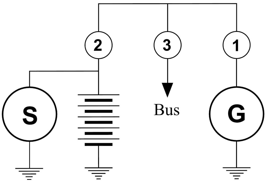
In aircraft, current measurement may be used in three locations (fig. 1) to monitor:

• the battery charging-discharging process at location 2, where a bidirectional sensor is necessary,
• the power generation at location 1,
• the power consumption by the various devices installed in the aircraft at location 3.

There is no need to measure the transient very high current in the starter circuit. In a light aircraft, we are only concerned with direct current measurements of low or medium intensity (typically -20 to +20 A) and low voltage (most often 12-14V). Insulation is not required, all the elements share the same ground. The required accuracy is of the order of  0.1 A. Remember that low cost is a key concern of this Website.

Based on these requirement specifications, two sensor types may be considered: shunt-based and Hall-effect sensors. The voltage drop across a calibrated low-resistance shunt is measured for the first type. For the second one, the Hall effect sensor produces an output voltage depending on the magnetic field generated by the current, and this voltage is measured. In both cases, the output voltage is very low and needs to be amplified.

Hall-effect sensors

Breakout boards equipped with low-cost Hall-effect sensors are widely available, most of the time with Allegro Microsystem chips. For example, see here or there. These sensors fully meet our requirements; they are straightforward to implement, accurate, and some are bidirectional. The main concern with these sensors is the tiny conductor inside the chip through which the total current flows. This raises a severe potential safety issue. What could happen if the chip became overloaded or, even worse, fried?  An electrical power failure in an aircraft is a very unpleasant situation… This is why we did not select these sensors.

Some Hall-effect sensors are specifically designed for aircraft. For example, see here. They do not raise the same safety issue as the previous ones. But they are clearly more expensive. Moreover, the wire positioning relative to the sensor seems rather approximative, which may lead to inaccurate or unreproducible measures. We do not have any experience with these sensors.

Shunt based sensors

Virtually all ammeters installed on aircraft are actually shunt-based. The only drawback of this current measurement technique could be the voltage drop across the shunt and the inherent power loss. Let’s consider a 20A/50mV shunt, a widespread model found on many aircraft; its resistance is only 2.5 milliohms. The maximum voltage drop is only 50 mV for a 20 A current, and the power dissipated in the shunt never exceeds 1 W. Such a voltage drop affects the aircraft’s electrical circuits only to a negligible extent.

As mentioned above, the voltage across the shunt is very low; it can not be directly measured by the analog-to-digital converter (ADC) of a microcontroller and needs to be amplified. This raises the question of the shunt and amplifier location. There are two methods of current sensing: low side and high side (fig. 2)

Shunt location and amplifier selection

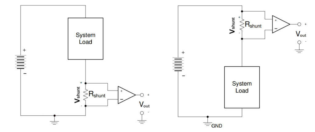
High-side current sensing offers two advantages when compared to low-side current sensing. It does not create ground disturbances and can detect a load short to ground condition (see reference here). So we have chosen the high-side technique.

This type of current sensing method requires that the amplifier be able to withstand high voltage. Among many others, we have selected the Texas Instrument LMP860x devices for the following reasons: they are mono or bidirectional single-supply voltage current sensing amplifiers with various precise fixed gains, and the path between their two stages is brought out on two pins to enable the option of modifying the gain. So they are particularly adequate in our applications to drive an ADC to full-scale value.

EMS current sensing circuit

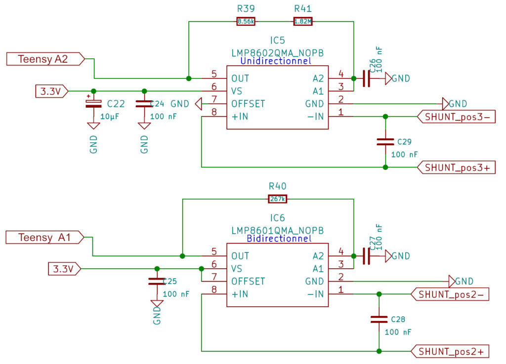
In the EMS, our choice was to monitor the current in locations 2 and 3, as defined in figure 1. A 50 mV/20A Murata shunt was mounted at both sites. The current monitoring input stage of the EMS is shown in figure 3.

For location 2, the current is bidirectional, and we choose to measure the -20 to +20A range. The measurement span is then 40A, i.e., 100 mV. With a gain of 32, 100 mV between the input pins gives 3.2 V on the output pin of the amplifier, which is almost the full scale of the Teensy ADC. The LMP8601 has a fixed gain of 20x. This gain needs to be increased to 32x by adding a resistor (R40, fig. 3) between the amplifier output (IC6 pin 5, fig. 3) and the input of the buffer amplifier (IC6 pins 3 and 4). This resistor creates a positive feedback that increases the gain. Please see LMP860x datasheet page 24 to calculate the resistance R of R40. The equation is:

R = 10⁵ x (G/(G-20))

Where G is the desired value of the gain. For G=32, this gives 267 kΩ. The current is bidirectional, so the offset pin (pin 7) is connected to the positive supply rail (3.3 V).

For location 3, the current is monodirectional, and we choose to measure the 0 to +20A range. The measurement span is then 20A, i.e., 50 mV. With a gain of 64, 50 mV between the input pins gives 3.2 V on the output pin of the amplifier. The LMP8602 has a fixed gain of 50x. This gain needs to be increased to 64x by adding a resistor (R39 and R41 in series, fig. 3) between the amplifier output (IC5 pin 5, fig. 3) and the input of the buffer amplifier (IC5 pins 3 and 4). For the LMP8602, the equation is:

R = 4 x 10⁵ x (G/(G-50))

For G=64, this gives 1.828571 MΩ. So we selected the following values: 8.56 kΩ for R39 and 1.82 MΩ for R41. The current is monodirectional, so the offset pin (pin 7) is grounded.

Software

The code that converts the amplifier output voltage to current in amps is as follows. This is an excerpt from our EMS software.

#define pinIP3unidir A2
#define pinIP2bidir A1

float VpinIP3unidir, VpinIP2bidir, Ibus, Ibat;

void setup() {
  //..............
  pinMode(pinIP3unidir, INPUT_DISABLE);
  pinMode(pinIP2bidir, INPUT_DISABLE);
  //...............
}

void loop() {
  /.................
  int digitalValueA  = analogRead(pinIP3unidir);
  VpinIP3unidir = digitalValueA*3.3/1023.0;
  //0 volts ---> 0A et 3.2 volts -> 20A d'où 3.3 volts -> 20.625A, donc 
  Ibus=(VpinIP3unidir*20.625)/3.3; 

  int digitalValueB  = analogRead(pinIP2bidir);
  VpinIP2bidir = digitalValueB*3.3/1023.0;
  //3.2 volts -> +20A et 1.65 volts -> 0A, d'où 0.1 volts -> -20A, et 0 volts -> -21,29A, et 3.3 volts -> 21,29A, donc
  Ibat=((VpinIP2bidir-1.65)*21,29*2)/3.3; 
  //.......................
}

In the EMS, the output of IC6 (bidirectional current sensing at location 2) is connected to the analog A1 pin of a Teensy 4.1 board. The analogRead() instruction on this pin returns a 10-bit digital value between 0 and 1023. This digital value is converted to a voltage value between 0 and 3.3 volts in the subsequent line. This voltage is then converted into a current value in amperes.

In bidirectional mode, with a 3.3 volts single supply, the output signal is mid-rail referenced, i.e., 3.3/2 or 1.65 volts. This reference corresponds to the middle of the chosen current range (-20 to +20A), i.e., 0 amperes. Remember that we decided to maintain a small safety margin when selecting the amplifier gain so that 20 amps give 3.2 volts on the output; therefore -20A give 0.1 volt. We easily deduce that a zero voltage output corresponds to -21.29A, and 3.3 volts correspond to +21.29A.

A similar calculation makes it possible to convert the 0 to 3.3 volts range IC5 output voltage into a unidirectional current value at point 3, in the 0 to +20.625 amperes range.