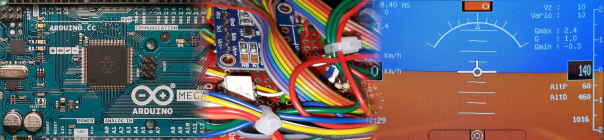
(EFIS pressure sensors: last updated by Benjamin on April 29, 2024)
The AvionicsDuino EFIS uses two pressure sensors: an absolute (or barometric) sensor to measure the ambient static pressure and a differential sensor to measure the dynamic pressure, which is the difference between the static pressure and the total pressure at the tip of the Pitot probe. The EFIS can then calculate the altitude based on the static pressure and the speed of the aircraft based on the dynamic pressure.
Principles of pressure sensors
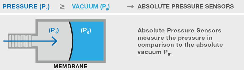
Absolute pressure sensors have a single port and measure pressure relative to absolute vacuum. They can be represented schematically as two compartments separated by a gas-tight membrane (Fig. 1). The pressure to be measured, P1, is applied to one side of the membrane, while in the other compartment, there is an absolute vacuum, therefore zero pressure P0. The deformation of the membrane reflects the pressure applied to the port.
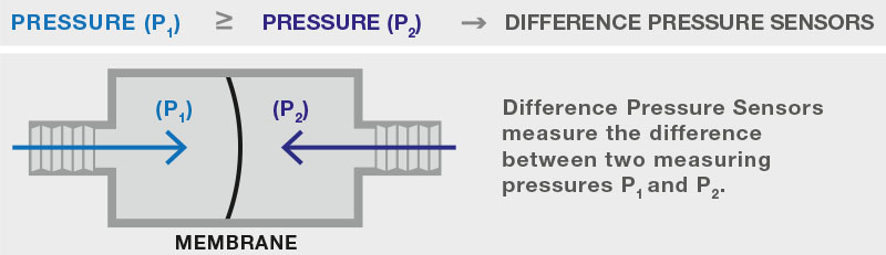
Differential pressure sensors have two ports. They measure the pressure P1 of one compartment in relation to that of the other, P2 (Fig. 2). The membrane deformation reflects the pressure difference between the two ports. Care must be taken regarding which port the higher and lower pressure can be connected to.
Characteristics of the sensors used in the EFIS
We use sensors from the AMSYS company. These are references AMS5915-1500-A for absolute pressure and AMS5915-0050-D for differential pressure. The membrane and the two compartments in the diagrams above are a convenient analogy to explain the basic principle of pressure sensors. In reality, these sensors combine a high-quality, membrane-based piezoresistive silicon sensing element with a modern mixed-signal CMOS application-specific integrated circuit (ASIC) on a ceramic substrate. The ASIC takes care of signal conditioning to offer a digital output with an I2C interface.
The choice of digital sensors was obvious due to their ease of use, reliability, precision, and accuracy, although the cost is higher than that of analog sensors. In addition, these digital sensors are calibrated and temperature compensated (thanks to an integrated temperature sensor), and they offer an output corrected for linearity deviations. They offer an excellent 14-bit resolution. All this is possible thanks to the microcontroller they include and the EEPROM, which allows individual factory calibration settings to be saved. Therefore, the advantages over an analog sensor are obvious.
An important selection criterion for these sensors was also the presence of ports that were easy to connect to the aircraft’s static and total pressure lines.
Choice of the sensor used for altimetry
In the AMS5915 series, we had the choice between two pressure ranges for altitude measurements: 700 to 1200 mbar or 0 to 1500 mbar. The first choice would theoretically have allowed better altitude resolution between 0 and 3000 meters (i.e., 10,000 ft or 700 hPa) but did not allow altitudes higher than 10,000 ft to be measured.
Therefore, we chose the AMS5915-1500-A sensor (0-1500 mbar) as it allows us to measure altitudes between 0 and 5,000 meters (16,666 ft) that the MCR Sportster may reach. Thus, pressure measurements between 1040 hPa at sea level and 540 hPa at 5,000 meters/16,666 ft are possible. So, only 500 hPa out of the 1500 full range is possible, or 1/3 of the range.
What altitude resolution does this allow to achieve? In the datasheet, we can read that the full span output (FSO) of the AMS5915 series sensors (i.e., the algebraic difference between the output signal at the maximum specified pressure -14,745 counts-, and the signal output at the minimum specified pressure -1,638 counts-) is 13,107 counts (instead of the 16,384 that one would expect with “full” 14-bit resolution).
A third of the FSO represents 13,107/3 counts, that is, 4,369 counts. So, for altitudes from 0 to 5,000 meters (16,666ft), we can calculate a theoretical altimeter resolution of 16,666/4,369=3.8 ft or just over one meter. The theoretical altitude resolution that this sensor makes it possible to achieve is, therefore, amply sufficient and much greater than the resolution of a traditional analog needle altimeter.
Choice of the sensor used for speed measurements
To choose the right sensor, it is necessary to first calculate the differential pressure obtained at the VNE of the aircraft, i.e., 320 km/h (173 knots, or 89 m/s) for the MCR Sportster. At this speed, the Mach number is well below 0.3, so we can consider the flow regime as incompressible and, therefore, use the simple formulation of Bernoulli’s theorem:
V2 = 2Pd/1.225
where :
– V is the speed in m/s,
– Pd is the differential pressure between the static pressure and the total pressure, expressed in Pascals,
– 1.225 is the density of air in standard conditions at sea level, expressed in kg/m3.
At a speed of 320 km/h, or approximately 89 m/s, the differential pressure will therefore be:
Pd = 89 x 89 x 1.225 / 2 = 4,852 Pa, or 48.5 mbar
The AMS5915-0050-D sensor, capable of measuring differential pressures between 0 and 50 mbar, is therefore perfectly suited to the MCR Sportster. This aircraft uses almost the entire sensor’s pressure range.
What speed resolution does this allow to achieve? The FSO (0 to 50 mbar) is 13107 counts, as with all AMS5915 series sensors. Using the equation above, we can calculate that a differential pressure of 50 mbar corresponds to a speed of 325 km/h. Therefore, the theoretical resolution is 325/13107, or 0.02 km/h. Given this excellent resolution, which even greatly exceeds essential requirements, we can see that this same sensor is also well suited to slower aircraft.
Testing AMSYS sensors
Two sensors in service in an EFIS were tested in real conditions, in flight. Two other sensors, recently acquired, especially for the occasion, were tested on the bench.
Flight tested sensors
The flight tests of the pressure sensors consisted of comparing the speed and altitude values of the AvionicsDuino EFIS with the corresponding values of a Dynon EFIS D10A installed on the same aircraft. These comparisons are shown at the bottom of the EFIS page.
In-flight and ground speed testing (differential pressure sensor)
Prior to installation, a zero point error of the AMS5915-0050-D differential sensor was noted. Its output signal for a differential pressure of zero was 15,69 counts instead of the 1,638 counts specified in the datasheet. On the other hand, for a differential pressure of 50 mbar, we obtained values very close to the 14,745 counts specified in the datasheet. Therefore, we modified the digOutPmin constant in the AMS5915_simplified library of the EFIS software accordingly to replace the value 1,638 with 1,569 (line 32 of the AMS5915_simplified.cpp file). For a sensor without this zero point error, the value of the digOutPmin constant must be 1,638.
A little utility that allows you to display the number of counts output from the AMS5915-0050-D sensor for any differential pressure between 0 and 50 mbar is available for download from the EFIS GitHub repository. This is the test_AMS5915-0050-D_sensor.ino file in the util folder.
For the flight tests, we had previously checked the accuracy of the data from the other existing speed indicators in the aircraft as rigorously as possible.
Checking of the aircraft’s existing speed indicators
Firstly, on the ground, using a water manometer, we ensured the accuracy of the speeds indicated by the Dynon D10A and by the TSO’d Winter anemometer, which is installed right next to it (fig. 3, 4, 5, and 6).
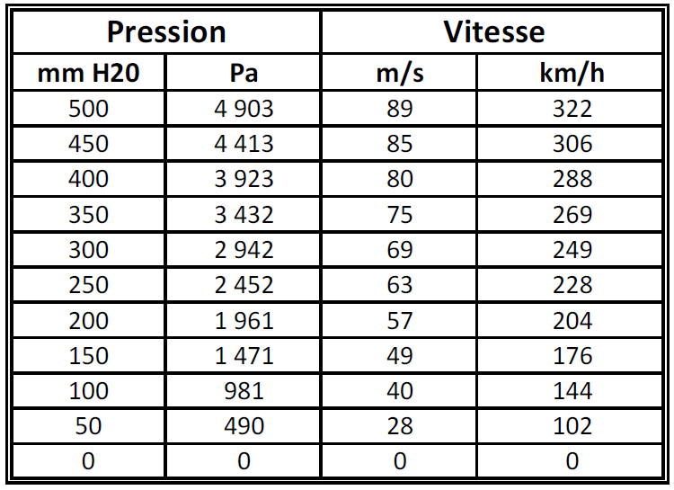
Using the formulas mentioned above, we can calculate the indicated airspeed (IAS), which should be read on the instrument by applying a given pressure on the Pitot probe (fig. 3)
Using a water manometer and a syringe, a known pressure is applied to the Pitot probe (Fig. 4). This is exactly the same system used for calibrating pressure sensors, which is shown schematically in Figure 9. Incidentally, this same system also allows for checking the strict tightness of the Pitot line.
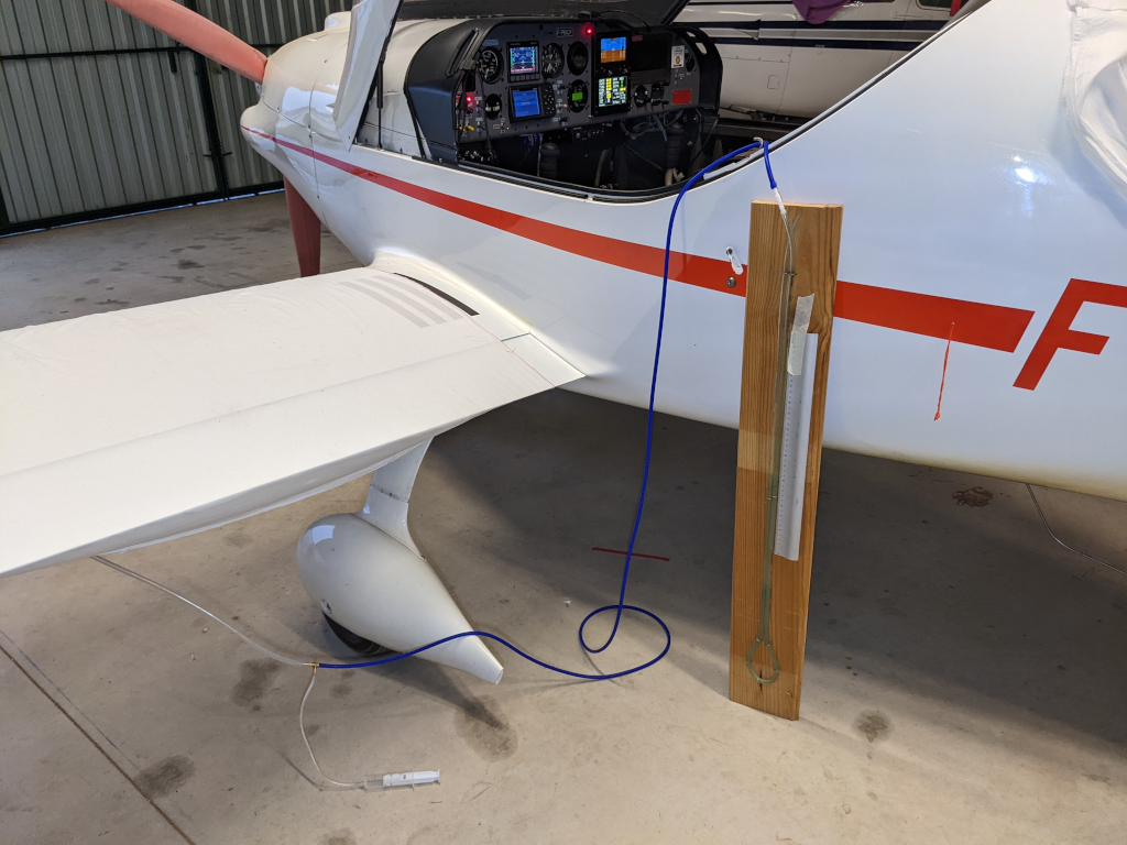
Figure 5 below shows that the value of the applied pressure is 300 mm H2O.
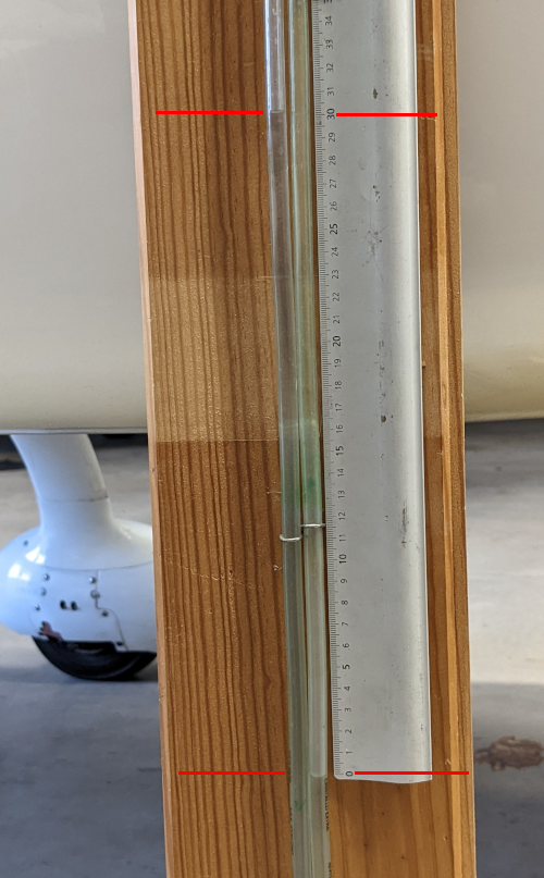
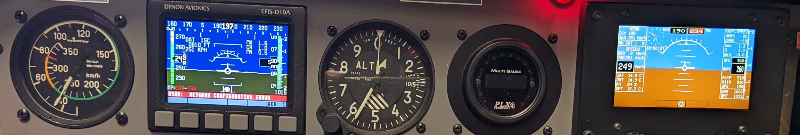
This pressure of 300 mm H2O corresponds to an IAS of 249 km/h (table in Figure 3). We see in Figure 6 below that the airspeeds indicated by the Dynon EFIS D10A and by the AvionicsDuino EFIS are identical and strictly equal to the calculated value, namely 249 km/h. You have to hover the mouse cursor over the photo to enlarge it.
Consistency check
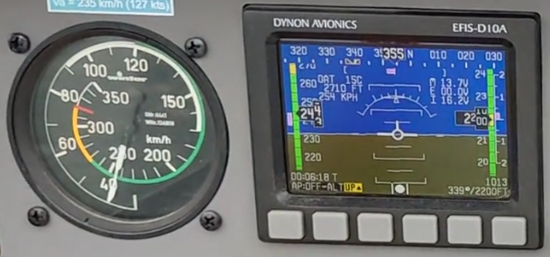
We also checked the consistency of the airspeed indications provided during flight by the Winter airspeed indicator and the Dynon EFIS (fig. 7).
In-flight checking using the GPS three-legs technique
Finally, we also checked the accuracy of the aircraft’s true airspeed (TAS) using the GPS 3-legs technique (references here and there). The TAS is calculated from IAS, altitude, and temperature. This technique is also a good way to check the accuracy of the static pressure and, therefore, the correct location of the aircraft’s static pressure ports.
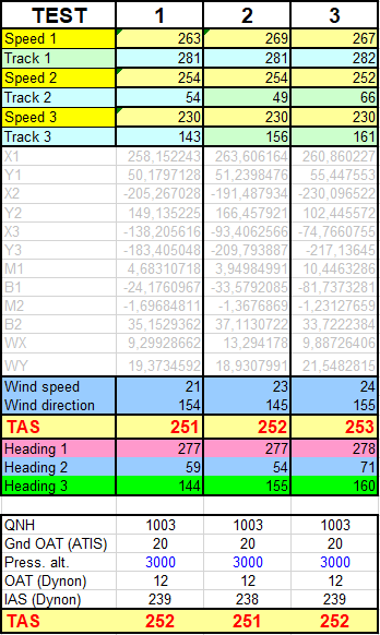
Figure 8 below shows the results of three TAS control tests using the GPS 3 legs technique. The upper part of the first box corresponds to the ground speeds and the GPS tracks that were recorded on three different tracks during each test. The intermediate calculations are shown in gray in the middle part. The resulting wind speeds and directions, TAS, and headings are shown at the bottom. The second box contains readings of altimeter data, external temperatures, and indicated airspeeds. The bottom line shows the corresponding calculated TAS. We see that the indications from the aircraft’s instruments are very close to the GPS-derived results.
From all the previous tests, we can conclude that the aircraft’s instruments are very accurate. Figure 13 on the EFIS page shows perfectly identical speeds between the Dynon and AvionicsDuino EFIS. This validates the differential pressure sensor used and the related calculations. Therefore, no other software correction than the modification of the digOutPmin constant was necessary.
In-flight and ground altimeter testing (absolute pressure sensor)
The software adjustment of the altitude calculation was a little more complex. On the ground, when setting the QNH on the Dynon and AvionicsDuino EFIS, the correct altitude of the airfield was displayed on the Dynon, but we always obtained a small error in the AMSL altitude read on the EFIS AvionicsDuino. This difference was always constant in sign and absolute value.
Ground correction
This difference was therefore taken into account by introducing the PrsCor menu option in the GEN menu of the EFIS. This option allows you to add a constant offset, in the form of the global pressureCorrection variable, to the pressure variable. The latter is the static pressure measured by the absolute pressure sensor. To adjust the PrsCor menu option on the ground without using another altimeter, you must know the local QNH and the exact AMSL altitude of the airfield.
By setting the QNH to the known value, PrsCor must then be adjusted with the rotary encoder until the correct airfield altitude is read. It may be necessary to carry out several tests on different airfields, on different dates, and with different QNH values, each time noting the error in order to average the necessary correction. Indeed, the QNH provided by ATIS or air traffic control is subject to small measurement errors, and it only offers accuracy to within 1 hPa, or 28 ft altitude.
In-flight correction
Figure 11 on the EFIS page shows the comparison between altitudes indicated by the Dynon and AvionicsDuino EFIS during a climb from the ground to 5000 ft. Several similar tests highlighted a minimal excess altitude on the AvionicsDuino EFIS compared to the Dynon. The error value was proportional to the altitude (span error).
We postulated that the Dynon displayed an exact value, so we introduced into the AvionicsDuino software a correction coefficient, in the form of the altitudeCorrection variable, equal (for our EFIS) to 0.995 (therefore to correct a very small error of the order of 0.5%). See line 217 of version 3.01 of the EFIS program. All altitudes calculated by the AvionicsDuino EFIS are multiplied by this coefficient before being displayed on the screen.
Comparative data
As indicated above, we assumed the accuracy of the Dynon EFIS’s altitude indications for these comparisons. Actually, the aircraft used for the tests has three other altimeter comparison points, which made it possible to make this postulate without too much fear of error: a conventional analog altimeter, the altimeter integrated into the transponder, and the altitude provided by GPS.
In the absence of these four means of comparing AvionicsDuino EFIS altimeter data in flight, the accuracy of this data would have been more difficult to demonstrate. Taking measurements in another aircraft requires being able to connect the altimeter to be tested to the static line. Taking the altimeter to test during a mountain trip is an option, provided you are in a mountainous area. Knowing the altitude of the place (mentioned on the maps) and the regional QNH makes it easy to test an altimeter. We will see further down on this page how to check an altimeter on the ground with a water manometer.
This gives us the opportunity to remind the reader of the importance of 1) the warnings on the AvionicsDuino Website home page and 2) compliance with the regulations. For data as important to flight control as speed and altitude, having redundant instruments is cautious and, in some cases, mandatory.
Sensors tested on the bench
Two new, recently acquired sensors were used for these tests: an AMS5915-0050-D for differential pressure and an AMS5915-1500-A for absolute pressure.
Testing the AMS5915-0050-D differential sensor
The water manometer
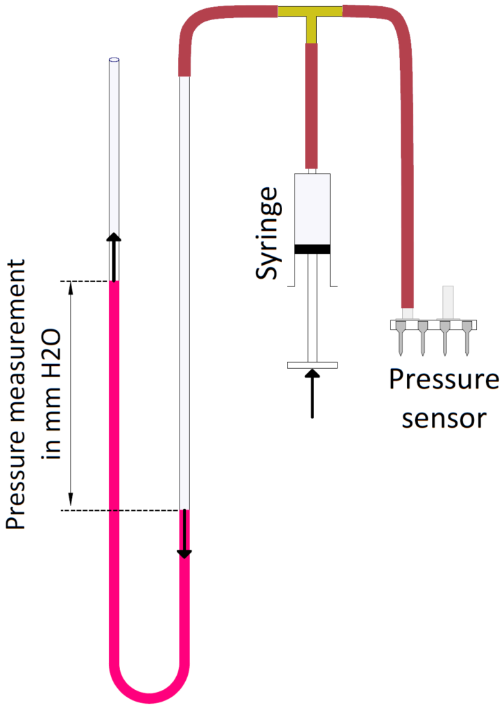
For this test, we made and used the water manometer schematized below in figure 9. A clear U-shaped plastic tube is partially filled with water, possibly with a dye added. This tube is positioned vertically. A ruler graduated in millimeters allows for measuring the difference in height of the levels in the two branches of the U (see also figures 4 and 5 above).
One end of the tube is open to atmospheric pressure, while the other is connected to the higher pressure port of the differential pressure sensor to be tested. The other port is open to atmospheric pressure. A T-connector is inserted between the manometer and the pressure sensor to connect a 20 ml syringe that allows the pressure to be measured to be applied to the system.
Experimental set-up
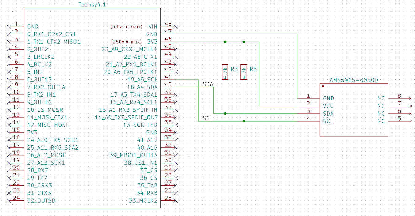
The pressure sensor was connected via I2C to a Teensy 4.1 board (fig. 10). Any Teensy or Arduino board would do the trick.
Test methodology
The Teensy 4.1 board used in our example was powered via USB by a PC. The test utility software mentioned above was uploaded to the Teensy board (test_AMS5915-0050-D_sensor.ino). The results were displayed on the serial monitor of the Arduino IDE. We thus noted the number of counts for different pressure values distributed throughout the entire measurement range of the sensor.
Results
The results of the 43 measurement points were entered into Microsoft Excel. We obtained the graph in Figure 11. Hover the mouse cursor over the graph to enlarge it.
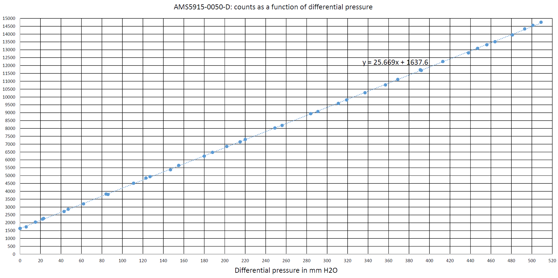
We see in Figure 11 that the response of the sensor is linear over the entire extent of its measurement range. The equation for the trend line is displayed on the graph. It shows that this line crosses the Y-axis almost exactly at 1638 counts, which is the expected value for zero differential pressure. We also see that for a pressure of 510 mm H2O, or 50 millibars, i.e., the maximum pressure specified, the number of counts is in the immediate vicinity of the 14745 counts expected in the datasheet.
It can be concluded that the sensor studied is excellent in accuracy and precision. The dispersion of the measurements around the trend line is very low. The attentive reader will, however, have noticed that the digital filtering provided by the test software improves this precision. This sensor showed no zero shift, span, or linearity error.
Testing the AMS5915-1500-A absolute sensor
The choice of the manometer to use
The practical problem for the absolute sensor is a bit more complex because the theoretical range of pressure to study is wider, around 500 hPa, as we saw above. If we chose to use a water manometer, this would represent a water column of more than five meters, which is not easy to implement.
Things would be simpler with a mercury manometer, but this type of manometer becomes rare, and its accuracy is much lower than that of the water manometer. The ideal would be to be able to use a high-precision laboratory pressure gauge, but this tool is not widespread, expensive, and rarely accessible to amateur aircraft builders. Finally, ordinary commercial pressure gauges are far from having the required precision.
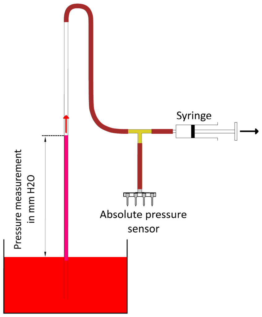
We nonetheless decided to use a water manometer because of its high precision and accuracy, but we limited the measurements to a water column of only three meters. This represents an altitude of around 3000 meters (or 10,000 ft), which is already substantial; most VFR flights take place below 10,000 ft. The experimental setup is shown in Figure 12. The principle is essentially the same as previously but adapted to a high negative pressure and, therefore, a much greater water height.
A clear, rectilinear vertical plastic tube 3 meters long plunges at its lower part into a large-capacity tank, open to atmospheric pressure and containing water (possibly colored). By pulling on the piston of a syringe connected to the top of this tube, a negative pressure is established relative to atmospheric pressure. The height of the column of water rising in the vertical tube makes it possible to measure this negative pressure. A T-connector connects the absolute pressure sensor to the system. The quantity of water rising in the vertical tube must be negligible compared to the capacity of the tank so as to maintain a constant level in the tank, which facilitates measures.
Test setup and methodology
For this test, the pressure sensor was connected via I2C to a Teensy 4.1 board powered by a PC’s USB socket. The results obtained were displayed on the serial monitor of the Arduino IDE. The experimental setup was identical to that of Figure 10.
The utility software used to display the absolute pressure measured in Pascals and the number of counts output from the AMS5915-1500-A sensor can be downloaded from the EFIS GitHub repository. This is the test_AMS5915-1500-A_sensor.ino file in the util folder.
Results
A series of 64 measurement points were carried out by applying variable negative pressure between 0 and -3000 millimeters of water. For each negative pressure value, we noted the number of counts, the absolute pressure in pascals measured by the AMS5915-1500-A sensor (calculated from the number of counts), and the absolute pressure measured by the water manometer.
This last measurement results from a calculation taking into account, on the one hand, the negative pressure measured by the water manometer and, on the other hand, the atmospheric pressure of the moment (QNH of an airport located 7 km away) and the topographic altitude of the place where the measurements were taken.
The measurements’ results were entered into Microsoft Excel to obtain the graph in Figure 13. You must hover the mouse over the graph to zoom in.
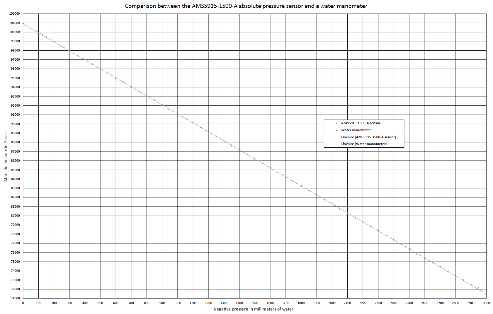
We note, on the one hand, the sensor’s linear response and, on the other hand, the almost perfect superposition of the trend lines representing the sensor’s measurements in pascals and the measurements made using the water manometer.
The graph below (fig. 14), taken from the same experimental data, shows the evolution of the sensor output in counts (Y-axis) as a function of the absolute pressure in millibars measured by the water manometer (X-axis).
The X-axis extends from 0 to 1500 millibars, which is the absolute pressure range of the AMS5915-1500-A sensor, and the Y-axis extends from 0 to 15,000 counts, which corresponds to the full span output (FSO) of the AMS5915 series sensors (as a reminder, the FSO is the algebraic difference between the output signal at the maximum specified pressure, here 1500 millibars, or 14745 counts, and the output signal at the minimum specified pressure, here 0 millibars, or 1638 counts).
The different measuring points are shown in red on the graph. The trend line, in dotted blue, extends across the entire measurement range. The measurements were made between 700 and 1000 millibars. The trend line extrapolates the results from 0 to 1500 millibars
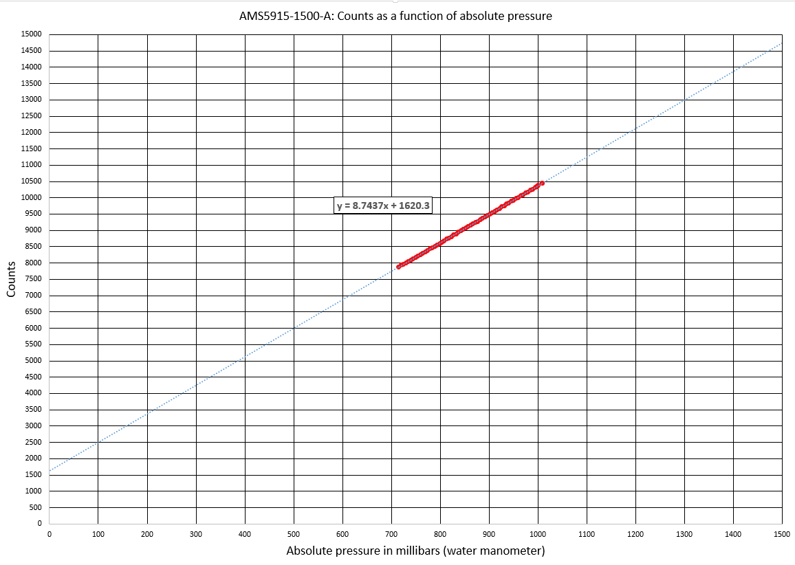
In Figure 14, we notice that the number of counts extrapolated for zero pressure is 1620, which is very close to the expected value of 1638. For 1500 millibars, the equation of the trend line makes it possible to calculate a number of counts equal to 14.736, which is also very close to the expected value of 14.745.
Here again, we can conclude from these experimental data that the absolute sensor studied is excellent in accuracy and precision. The dispersion of the measurements around the trend line is low. Moreover, this sensor showed no zero shift, span, or linearity error.
Conclusions
Pressure sensors, like all sensors, can be subject to errors that affect precision, accuracy, or both.
Precision reflects the greater or lesser dispersion of the values. It can be improved by filtering. The graphs obtained during the bench tests showed that the precision of the sensors tested is very satisfactory, the dispersion of the different measurement points on either side of the trend line is low.
Accuracy reflects the difference between a measurement and the real value of the measured quantity. The sensors tested on the bench were found to be very accurate. We have seen that certain sensors can suffer from inaccuracy. It is sometimes possible to correct this error satisfactorily using software, with the example of the differential sensor installed in the AvionicsDuino EFIS. A new differential sensor affected by a significant zero error (>1% of FSO), as we observed, should, however, be the subject of a warranty exchange request. Hence, there is a great interest in testing these sensors.
Digital pressure sensors equipped with ports that can be connected to an aircraft’s static and Pitot lines and whose prices remain compatible with a DIY project like the AvionicsDuino EFIS are rather rare.
Apart from the AMSYS sensors from the AMS5915 series that we chose for the EFIS, other manufacturers, such as Honeywell and TE Connectivity, offer digital sensors with similar characteristics and in approximately the same price range. The Honeywell MPRLS 0025PA absolute sensor is used in the AvionicsDuino EMS for manifold pressure measurement. We also tested a TE Connectivity differential sensor from the 4515DO series for a project currently being evaluated concerning the automatic regulation of the AFR (Air Fuel Ratio) on a Rotax 912 engine.