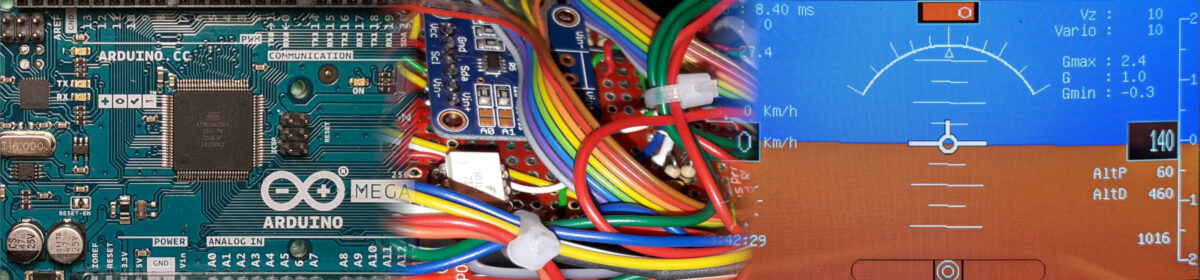
(Digital filter. Last updated by Benjamin on October 1, 2022)
In signal processing, the function of a digital filter is to remove certain parts of the signal, such as noise.
A microcontroller’s periodic reading of a sensor provides a series of values over time at a frequency determined by the software. Regardless of the sensor, microcontroller, software, or sampling frequency, the signal obtained is disturbed by measurement noise. This noise may be due to outside interference or the inevitable lack of precision in the sensor.
Remember that a sensor’s precision reflects the measurements’ dispersion around an average value. The accuracy reflects the greater or lesser proximity of this average value to the actual value being measured. In figure 1 below, the blue curve represents the signal to be measured, while the red curve corresponds to the noisy measurement of this signal. Note that a clear imprecision mars the measurements made by this sensor but that it has good accuracy since the distribution of the various measurements is centered on the actual value of the signal.
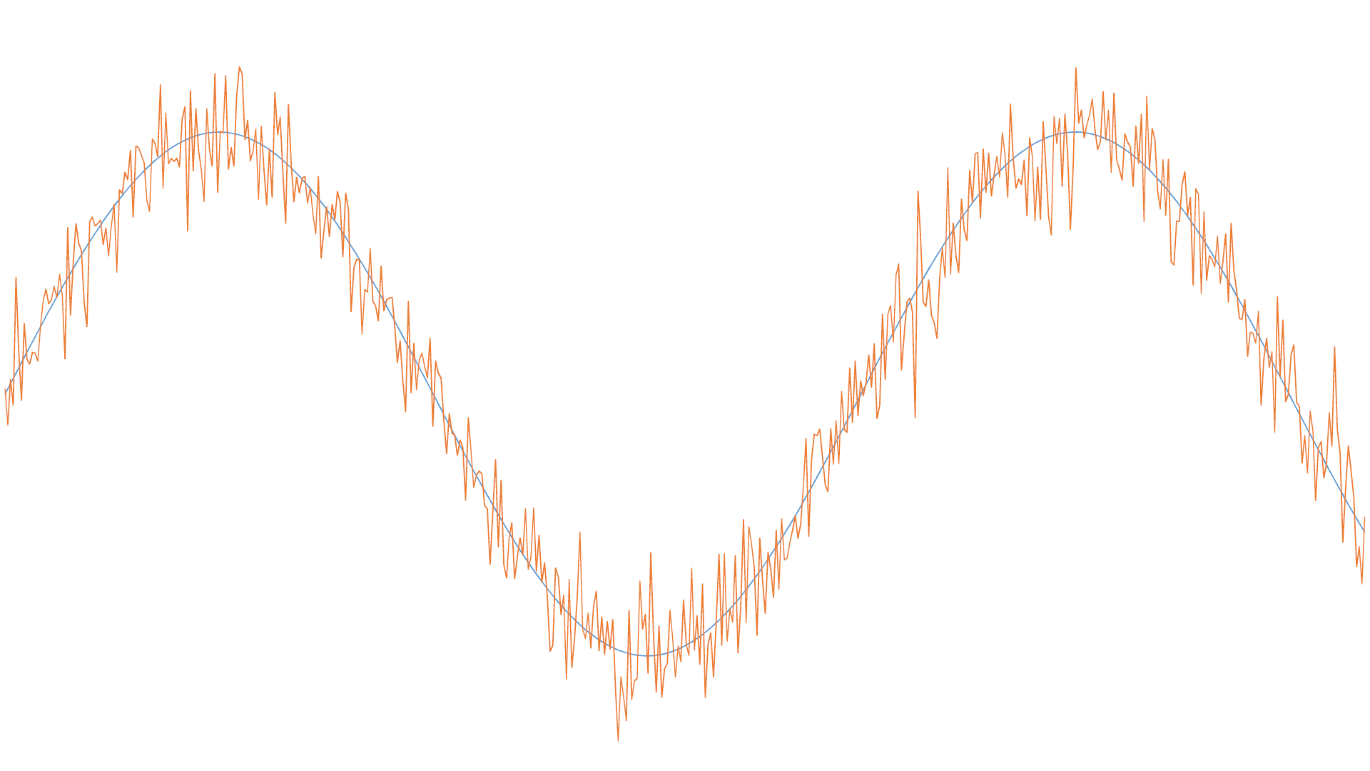
The noisy signal in figure 1 is very characteristic of what is usually encountered in avionics: whether it concerns the static pressure, the cylinder head temperature, the fuel flow, the main bus voltage, the pitch angle, the rate of climb, or the engine RPM, measured values generally change relatively slowly, while measurement noise has a much higher frequency, which is that of the sampling frequency. Smoothing techniques will therefore use a low-pass filter, i.e., a filter that removes high frequencies. The purpose of digital filters is to correct measurements in real-time, to come as close as possible to the ideal curve corresponding to the noiseless signal, and to display stable and precise values.
To achieve this goal, two simple low-pass filter techniques are used in the programs on this website: the moving average filter and the Infinite Impulse Response filter (IIR filter). The sketch to download below illustrates these two techniques; it runs on all Arduino and Teensy boards. It is beyond the scope of this website to present the complex mathematical theories of signal filtering. For further information, the reader may refer, for example, to this site and many others.
Moving average digital filter
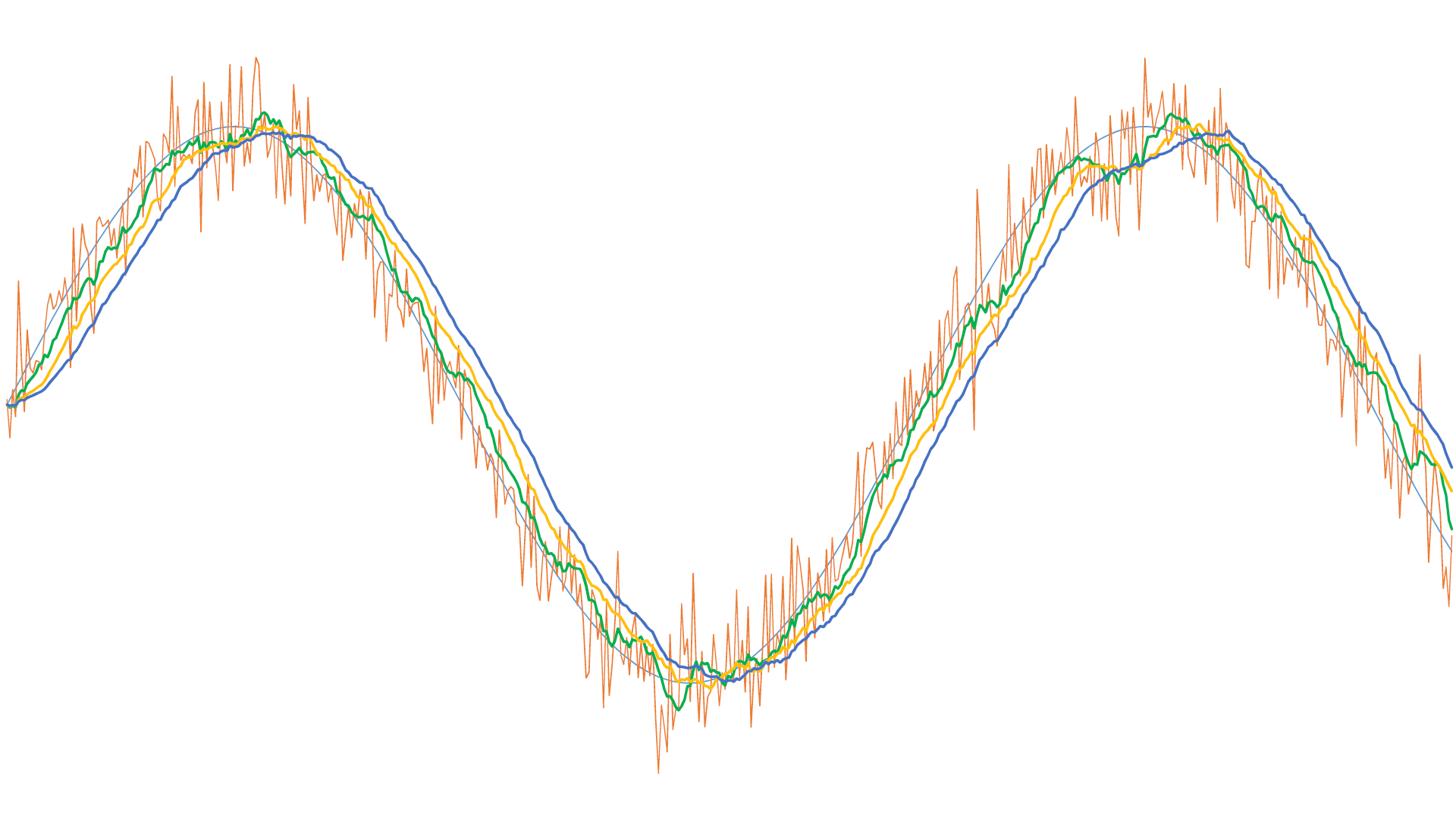
This filter consists of calculating the average of the current value and the N previous measurements for each measurement. This means storing in memory these N previous measurements. This is also referred to as a finite impulse response filter because this filter is based on a finite number of input signal values. The larger the number N, the better the filtering quality. The memory resources needed to store the N previous values may become an issue with 8-bit AVR microcontrollers. With increasing values of N, we will see a delay of the filtered curve with respect to the signal (phase shift). This delay is easy to estimate. It is equal to the product of the sampling period multiplied by N / 2. If the sampling period is 50 ms, and the moving average takes 20 samples into account, the delay will be 500 ms.
Figure n°2 shows the effect of this filter on the same signal as that of figure n°1 for different values of N. When implementing this type of filter, you must adapt the N to the noise amplitude: the more significant the noise, the greater N must be for good filtering, but the more evident the phase shift will be. A drawback of this very efficient filter is the (quite relative) complexity of the algorithm that implements it. It is always preferable to process a signal with as little noise as possible. The signal quality may sometimes be improved by changing the sensor model. Or by acting on external interference (shielding, ground loops, cable length, etc.).
Infinite Impulse Response digital filter
This is a recursive filter. The filtering of each new measurement includes the previous filtered value, along with a coefficient C, according to the formula:
Filtered value = previous filtered value * (1 – C) + current value * C
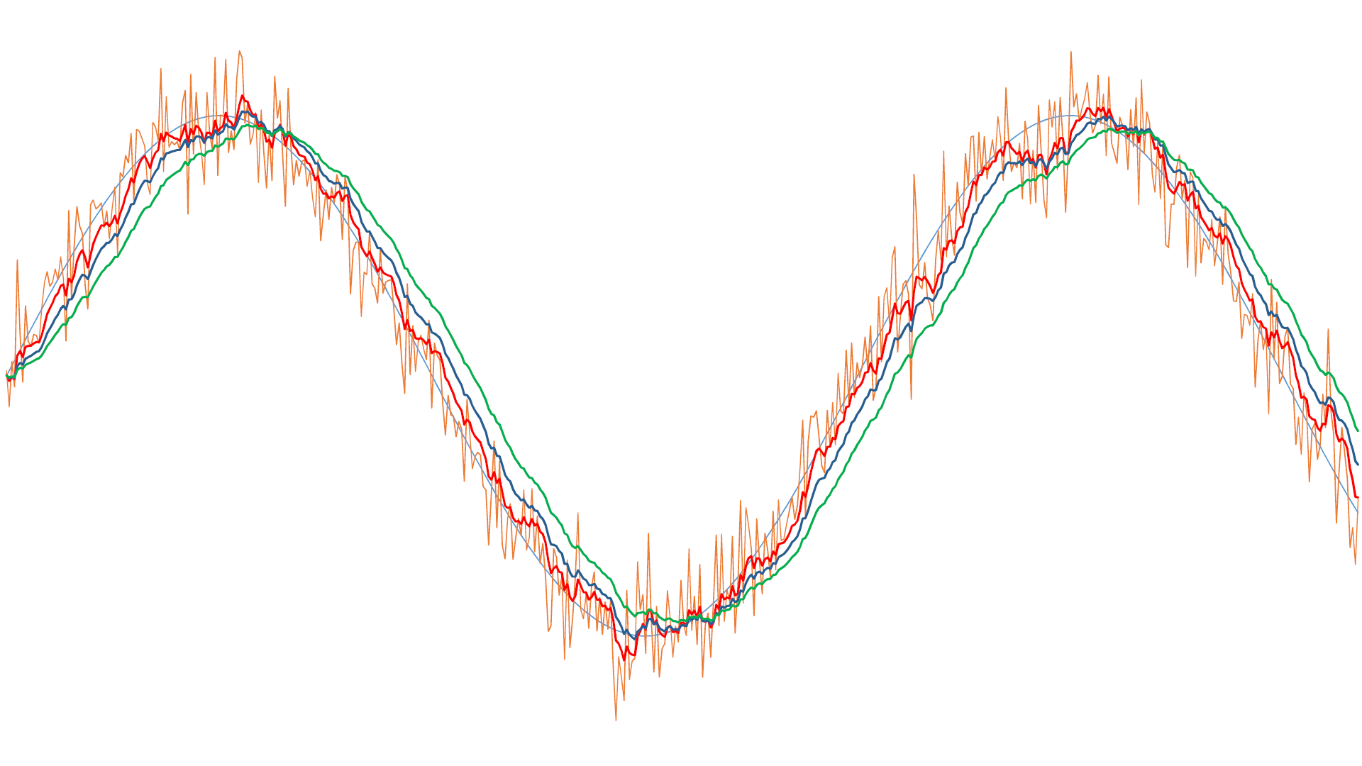
We speak of an infinite impulse response because all the previous values, since the start of the filtering, influence future filtered values in theory. In practice, this influence quickly becomes negligible with time unless the C coefficient is excessively low. For our current avionics applications, C generally ranges between 0.1 and 0.02. This filter’s advantages are its algorithm’s simplicity and the low memory resources needed. Only one value needs to be memorized between each sample. As for the moving average filter, a phase shift appears and increases when the filter coefficient decreases. This results in an improvement in filtering. We see in figure 3 the same noisy signal as in the previous figures, processed by this recursive filter, with different values of the C coefficient.
Comparison between these two filters
Figure 4 compares the same noisy signal, either filtered by a moving average filter on 30 samples or by an IIR filter with a coefficient of 0.06.
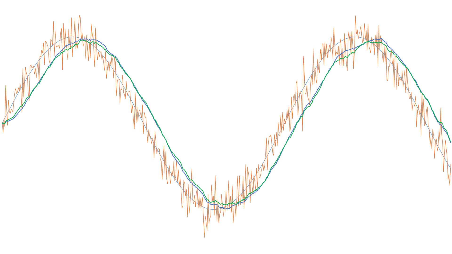
Figure 4: Comparison of the IIR filter with a coefficient of 0.06 (green curve), and the moving average filter on 30 samples (blue curve).
What can we conclude from this comparison? For this very noisy signal, figure n°4 seems to show a (very) slight advantage for the moving average filter (blue curve). The phase shift of the two curves is almost identical; the blue curve seems perhaps a little better smoothed, and its amplitude is similar to that of the non-noisy signal, while the amplitude of the green curve is a little “flattened.” The downloadable sketch above allows you to perform all the simulations you want to compare these two filters. You can vary the number of samples taken into account for the moving average, the coefficient of the IIR filter, and even the noise amplitude by increasing or decreasing its standard deviation.
The motivated reader may experiment with other filters, adding them to the same sketch. For example, the Kalman filter, for which there are libraries for Arduino and Teensy, here and there.
To choose the right filter and adjust its parameters, the preliminary study of the signal to be filtered is of the utmost importance. Recording a raw signal on a micro SD card in real (in flight) or simulated (in a car) conditions makes it possible to test various filters. Either with a spreadsheet like Excel or by “playing back” the signal on an Arduino or a Teensy and observing the curves using the serial plotter of the Arduino IDE. All the above curves were obtained with this serial plotter.