Digital compass

(Digital compass: Last updated by Benjamin on March 24, 2024)

The magnetic compass, the clock, the sextant, and the maps have long been the main navigation instruments, with the log in the navy and the anemometer in aviation that measure speed and allow estimates of distance traveled as a function of the elapsed time. Some World War II planes were equipped with an astrodome to allow the radio navigator to take an astronomical point with the sextant. At the end of the 1950s, Air France had equipped its Super Starliners with a periscopic sextant!

Radio navigation, then GPS, got the better of these almost ancestral navigation techniques. However, dead reckoning navigation, relying exclusively on the watch and the compass, is still taught. That is good because this base is essential for a student pilot to acquire a good mental representation of the time and space in which our aircraft operate. The pilot who has gained a little experience keeps his watch, but he no longer looks much at his magnetic compass. Except sometimes to reassure himself by thinking that he will be able to rely on it in the event of a failure of his GPS or tablet … on the condition of having kept the proper reflexes of dead reckoning navigation in mind!

Apart from regulatory obligations, the traditional magnetic compass has become of little use or even obsolete for some. However, it retains another interest in its digital version when coupled with a computer and a GPS. For example, to precisely indicate to the pilot the wind direction and speed, thanks to a calculation involving the aircraft’s true airspeed, the true course and ground speed provided by the GPS, and the magnetic heading provided by the compass, corrected for the magnetic deviation.

Earth’s magnetic field

The Earth’s magnetic field is established between the north and south magnetic poles, not to be confused with the geographic poles, hence the magnetic deviation. As with a simple bar magnet, magnetic field lines radiate from the south to the north magnetic pole, as shown in Figure 1.

This schematic representation shows that the field lines are roughly parallel to the earth’s surface around the equator, perpendicular to this surface around the magnetic poles, and more or less inclined depending on the latitude. But regardless of geographic location, the projection of a magnetic field line onto a plane parallel to the Earth’s surface is always oriented toward a magnetic pole (although it is necessary to take into account local variations of the magnetic field). This is the basic principle of the compass, an instrument that must always be horizontal to indicate the direction of the magnetic pole.

The magnetometer, the heart of a digital compass

The heart of a digital compass is a triaxial magnetometer. This particular sensor analyzes the surrounding magnetic field and breaks it down into three vectors along the three orthogonal axes x, y, and z of its Cartesian coordinate system.

There is a wide variety of magnetometers. Those that interest us within the framework of this site are of the magnetoresistive type. This technology makes it possible to obtain low-cost, precise, sensitive, and reliable sensors of infra-millimeter size. These sensors equip all smartphones on the market. These sensors are often associated with accelerometers and gyrometers within an IMU (Inertial Measurement Unit).

If a magnetometer is placed horizontally on a table, with the z-axis vertical, the x and y axes are, therefore, in a horizontal plane parallel to the Earth’s surface. In this case, analysis of the x and y components alone is sufficient to calculate the magnetometer’s magnetic orientation.

However, the magnetometer attached to an aircraft’s structure cannot always be horizontal. Consequently, the calculation of the magnetic orientation will have to involve the magnetometer’s three axes and integrate the aircraft’s pitch and bank angles.

For this project, we chose to use the LIS3MDL sensor from ST Microelectronics on an Adafruit board. This recent sensor communicates using the I2C or SPI bus. Several libraries are available.

Magnetometer calibration

The LIS3MDL is factory-calibrated for sensitivity and zero-gauss level. The corrective values are stored in non-volatile memory internal to the sensor. Each time the device is turned on, the parameters are loaded to the internal registers to be employed during active operation, which allows the device to be used without further calibration. Therefore, the user does not have to redo this particular calibration.

On the other hand, the user must meticulously calibrate the sensor to consider the particular magnetic environment at its final location in the aircraft. Indeed, this environment can more or less severely disturb the Earth’s magnetic field.

There are two sources of magnetic disturbances: hard iron and soft iron. To put it simply, hard iron refers to objects that produce a magnetic field, such as permanent magnets or current-carrying wires. Soft iron refers to certain metals such as iron or nickel, which, although not magnetized, can deflect the lines of the earth’s magnetic field. Many sites on the Internet explain 1) the theory of these disturbances, 2) calibration techniques, and 3) compensation methods.

Without going into complex mathematical theories, which are beyond us, we will practically approach points 2 and 3, which can help the reader to calibrate any magnetometer, i.e., to determine the coefficients necessary for the compensation. Then, we will explain how to introduce these compensation coefficients in an algorithm to obtain an exact magnetic heading despite the magnetometer environment’s hard and soft iron disturbances. It is then up to the user to consider the local magnetic deviation where he is flying to calculate the proper geographical heading.

The most evident precautionary measure is to install the magnetometer in the aircraft as far as possible from all sources of interference. For example, it could be installed in a wingtip, provided there are no strong current-carrying wires in the vicinity, for example, to feed flashing anti-collision lights.

The calibration procedure

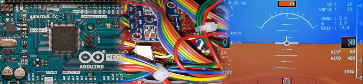
It consists of collecting, at best in the magnetometer’s future environment, a large number of measurements of the magnetic field on the three axes in all the sensor’s possible positions. To do this, after connecting the magnetometer to a microcontroller (Arduino, Teensy, or other), you need to upload an elementary sketch that sends the raw values of the magnetic field on each of the three axes to the Arduino IDE terminal.

All libraries offer this type of sketch as an example. You must adapt the sketch to obtain output data formatted according to the tool you will use to calculate the calibration parameters. Then, you have to start the sketch and manually rotate the sensor around all of its axes for approximately 30 to 60 seconds. Then, all you have to do is copy and paste the content of the terminal screen and save it in a “.txt” file. For example, we get this:

In this example, the tool used to calculate the calibration coefficients is the Magneto 1.2 software, which is downloadable here. The .txt file must be formatted (for example, with NotePad ++ or any word processing software and the “find-replace” function) to contain the magnetic field values on each line, separated by a space, on the x, y, and z axes.

Once the data has been saved, you must launch Magneto 1.2 and indicate the location of the text file to be processed. More explanations here, particularly for the entry to be made in the “Norm of Magnetic or Gravitational Field” box. It is necessary to proceed by successive approximations until the average of the three diagonal boxes circled in red on the screenshot below (Fig. 2) is as close as possible to 1.

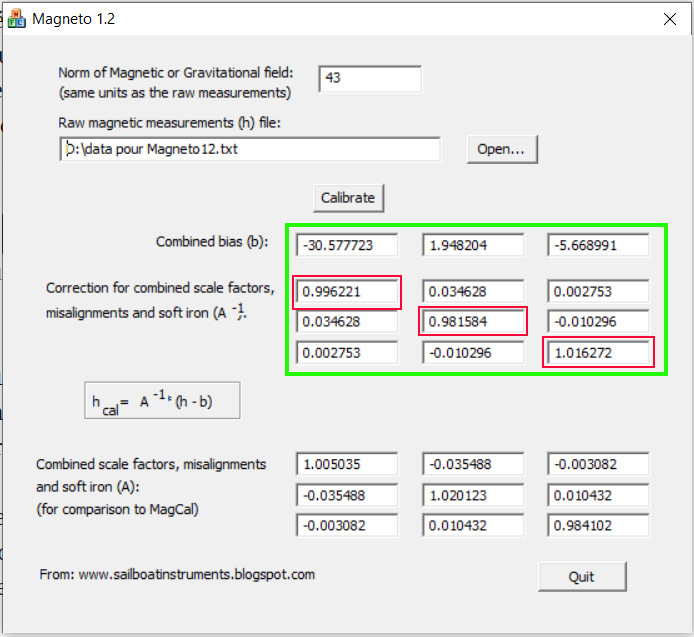
In the green frame of Figure 2, we have all the calibration coefficients we need to introduce in the sketch that manages the magnetometer to perfectly compensate for the hard and soft iron distortions.

These same coefficients can be obtained with another software: MotionCal, which is downloadable here. Depending on the operating system and antivirus protection used, MotionCal can sometimes be a little tricky to download, probably because it is an executable file hosted on an unsecured page of the PJRC Website. PJRC is the manufacturer of Teensy boards. Copying and pasting the URL of the download page (see below) into a new browser tab usually resolves the issue.

(http://www.pjrc.com/teensy/beta/imuread/MotionCal.exe).

The principle of MotionCal is slightly different. This software uses the magnetometer data received on the serial port in real time without having to save them in a file. To do this, you must close the Arduino IDE terminal and indicate in MotionCal which serial port to use. This is the one where the Arduino or Teensy board is connected.

Formatting the data output to the serial port is a bit more complicated than with Magneto 1.2, as MotionCal is designed to receive data from a 9 DOF IMU (triaxial accelerometer + triaxial gyro + triaxial magnetometer). If we take the first line of the file planned for Magneto 1.2, namely: “-52.27 -8.07 -40.49”, its formatting for MotionCal would be: “raw: 0,0,0,0,0,0,523,81,405”. The values ​​recorded on the three axes of the magnetometer are multiplied by ten and rounded to the nearest integer, preceded by six zeros, and separated by commas, with the word raw at the beginning of each line.

The imucal .ino example from the Adafruit library for the LIS3MDL implements this particular formatting. During the magnetometer’s rotational movements for calibration, a sphere gradually appears in the MotionCal graphics window. When the sphere is complete and centered, the procedure can be stopped, and the values ​​shown in the green frame can be noted (see Figure 3).

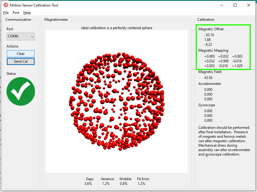
Magneto v1.2 and MotionCal tools each provide two matrices of decimal numbers, and their comparison shows that the two software provide almost identical coefficients. These coefficients are to be used in the application software operating the magnetometer to achieve the hard and soft iron compensation.

Of course, one can object to this calibration procedure, arguing that it only concerns the magnetometer itself, with the microcontroller directly attached to it, as well as the box that protects the assembly with its connections, but before fixing this assembly to the structure of the aircraft. The latter can, in fact, also generate magnetic disturbances.

However, it is generally not possible to quickly rotate the entire aircraft around its three axes, except during aerobatic maneuvers. Hence, the utmost importance is carefully selecting the magnetometer’s location, as far as possible from magnetic disturbances. However, it is possible to record the raw data of the magnetometers in flight, in all likely attitudes of the aircraft, according to its flight envelope, and in all headings. After the flight, this recording should be submitted to Magneto 1.2 or MotionCal to see if the coefficients thus obtained are different from those obtained by simply rotating the magnetometer housing manually, as described above.

The hard and soft iron compensation procedure

To process the calibration parameters obtained in the previous step, we must find the product of a 3 × 3 matrix by a 3 × 1 matrix. If necessary, the reader can refer to an elementary matrix algebra tutorial to understand the algorithm.

The calculation to be carried out is as follows:

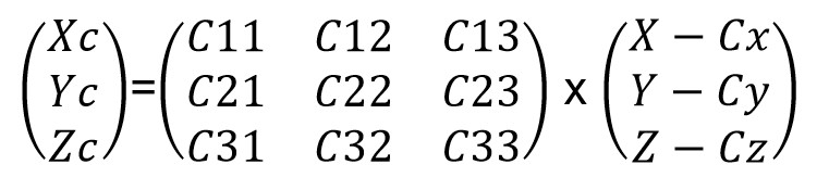
Where Xc, Yc, and Zc are the compensated values, C11 to C33, and Cx, Cy, and Cz are the coefficients calculated by MotionCal or Magneto 1.2, and X, Y, and Z are the magnetometer’s raw values.

If we take, for example, the raw values mentioned above, namely “-52.27 -8.07 -40.49”, and we want to apply a compensation to them with the coefficients in Figure 3, we have:

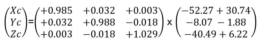
Then:

Xc= 0,985 x (-52,27+30,74) + 0,032 x (-8,07-1,88) + 0,003 x (-40,49 + 6,22) = -21,63

Yc= 0,032 x ( -52,27+30,74 ) + 0,988 x ( -8,07-1,88 ) -0,018 x ( -40,49 + 6,22 ) = -9,90

Zc = 0,003 x ( -52,27+30,74 ) -0,018 x ( -8,07-1,88 ) + 1,029 x ( -40,49 + 6,22 ) = -35,15

Example of the corresponding code:

#include <Adafruit_LIS3MDL.h>
Adafruit_LIS3MDL lis3mdl;
#define LIS3MDL_ADDRESS 0x1C

// Variables pour stocker les données brutes du magnétomètre
float magx, magy, magz;

// Données correctives issues de la calibration du magnétomètre. Ces données sont applicables à des mesures en µTesla.
float MagOffset[3] = {-30.74, 1.88, -6.22}; // Offsets pour les axes x, y et z
float mCal[3][3] = 
{
  {+0.985, +0.032, +0.003},
  {+0.032, +0.988, -0.018},
  {+0.003, -0.018, +1.029}
};

// Variables pour stocker les données magnétiques corrigées
float magxc, magyc, magzc;
float capmagnetique;

void setup() {
lis3mdl.begin_I2C(LIS3MDL_ADDRESS, &Wire1);
}

void loop() {
lis3mdl.read();      // Acquisition de X, Y et Z 
  magx = lis3mdl.x/68.42; //Conversion des données digitale brutes en µTesla
  magy = lis3mdl.y/68.42; //voir datasheet LIS3MDL p 8
                          // (https://www.st.com/resource/en/datasheet/lis3mdl.pdf)
  magz = lis3mdl.z/68.42;
  
// Calcul du produit des matrices
  magxc = mCal[0][0]*(magx-MagOffset[0])+ mCal[0][1]*(magy-MagOffset[1]) + mCal[0][2]*(magz-MagOffset[2]);
  magyc = mCal[1][0]*(magx-MagOffset[0])+ mCal[1][1]*(magy-MagOffset[1]) + mCal[1][2]*(magz-MagOffset[2]);
  magzc = mCal[2][0]*(magx-MagOffset[0])+ mCal[2][1]*(magy-MagOffset[1]) + mCal[2][2]*(magz-MagOffset[2]);

}

Computation of the magnetic heading

Once the magnetometer has been calibrated and the calibration coefficients applied to the raw values, we have the necessary parameters to calculate a magnetic heading.

In the simplest case, where the magnetometer is strictly horizontal, the z-axis is vertical, and its magnetic field component is not involved in the calculation. The magnetic heading (in degrees, from 0 to 360) can then be obtained very simply by the following two lines of code:

capmagnetique = atan2(magyc,magxc)*(180/PI);
if (capmagnetique<0) capmagnetique+=360;

However, this simple code is not appropriate for an airplane, where the roll and pitch angles must be considered. Therefore, the magnetic field component along the Z axis is involved, as well as the components along the X and Y axes. The roll and pitch angles are obtained from the AHRS in an airplane. One should not rely on the indications of a simple accelerometer because, in turn, the centrifugal force would not allow the latter to provide a vertical reference in the Earth’s reference frame.

Therefore, it is necessary to first perform a tilt compensation for the aircraft’s inclinations according to the roll and pitch axes. This calculation makes it possible to determine the two components Xh and Yh in a horizontal plane (in the Earth’s reference frame) as a function of Xc, Yc, and Zc, the triaxial components measured and calibrated above.

The equations are as follows:

• Xh = Xc * Cos(pitch) + Zc * Sin(pitch)

• Yh = Xc * sin(roll) * sin(pitch) + Yc * cos(roll) – Zc * Sin(roll) * Cos(pitch)

The code for obtaining an exact magnetic heading based on the attitude of the aircraft and the calibrated data from the magnetometer, therefore becomes:

Xh = magxc * cos(pitch) + magzc * sin(pitch);
Yh = magxc * sin(roll) * sin(pitch) + magyc * cos(roll) - magzc * sin(roll) * cos(pitch);
capmagnetique = atan2(Yh,Xh)*(180/PI);
if (capmagnetique<0) capmagnetique+=360;

The practical realization of the digital compass

Most magnetometers, like the LIS3MDL, have an I2C and/or SPI output. These interfaces are not intended to transmit signals over a great length. We have also seen that a good location must be away from magnetic disturbances, especially those related to the engine, DC power generation, and instrument panel.

For these reasons, we have chosen to combine a magnetometer and a microcontroller in a remote module (Fig. 4). Measurements are transmitted to the main EFIS module, located on the instrument panel, via a CAN bus. Indeed, this high-speed bus allows for long lengths and is excellently immune to electromagnetic interference.

The CAN Bus implemented in our project is particularly simple. It has only five nodes: the remote module described on this page, the main EFIS module, the AHRS, the EMS, and the Micro-EMS. Therefore, we have decided to bypass the complex constraints and recommendations of the CANaerospace protocol.

The location chosen in a wing tip is also conducive to installing a temperature and humidity sensor, which is necessary for calculating the density altitude. We have chosen the Adafruit “SHT-30 Mesh-protected Weather-proof Temperature / Humidity Sensor” module, product ID 4099.

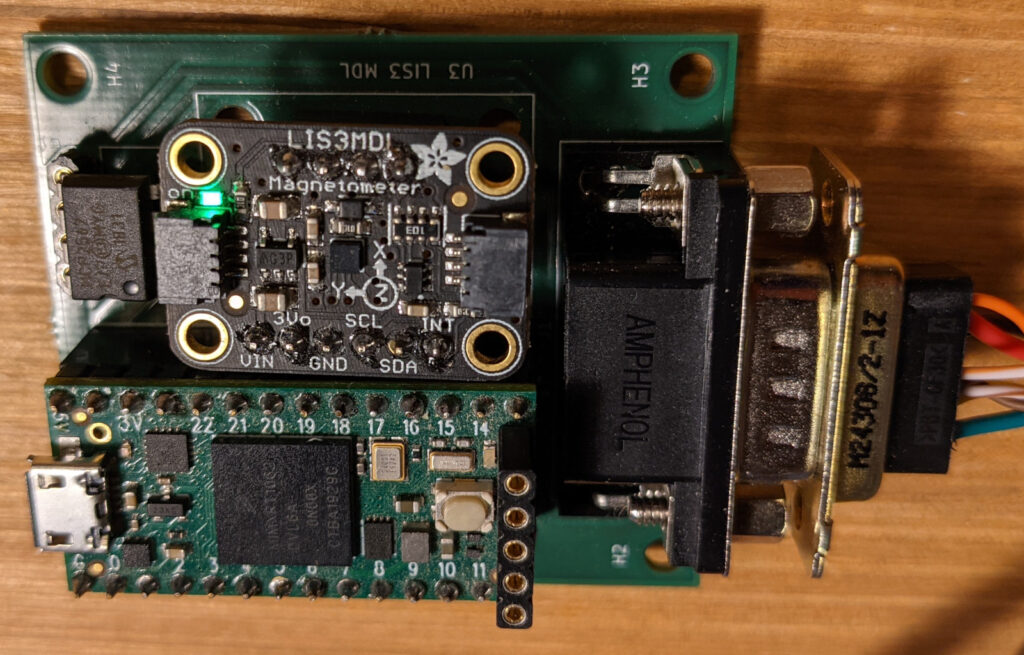
The microcontroller board is a Teensy 4.0, associated with an MCP2562EP CAN bus transceiver. Connections to the CAN bus and to the temperature and humidity sensor are made through a 9-pin D-SUB connector.

Just like the AHRS module, the digital compass module must be perfectly aligned with the aircraft’s roll, pitch, and yaw angles. To do this, you must power on the EFIS and very precisely position the plane’s wheels in height so that the artificial horizon is perfectly horizontal. A simple spirit level is then sufficient to align the magnetometer module horizontally to within 0.1° in pitch and roll (fig. 4).

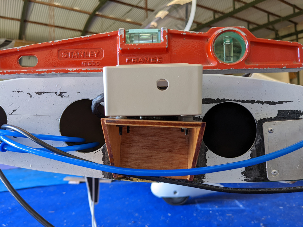
The orientation of the digital compass module (fig. 5) is as follows: the Teensy and LIS3MDL boards are on top, the LIS3MDL towards the front, and the D-SUB connector is on the right.

Download the source code on GitHub

Results

This remote module has been flight-tested with success. Everything works as expected. Compared to the Dynon EFIS, magnetic headings are identical to plus or minus 5 degrees, and outside air temperature is identical to plus or minus 0.5°C. Density altitude, the calculation of which involves outside air temperature and relative humidity, is difficult to compare with that displayed by the Dynon, which does not include a humidity sensor. It is generally within a range of plus or minus 250 feet with that of the Dynon, which is perfectly consistent with the influence of relative humidity.