(Rotax temperature sensors, last updated by Gabriel on October 13, 2022)
Temperature sensor theory
Temperature sensors used in our aircrafts (especially on Rotax engines) are thermistors made of a negative temperature coefficient (NTC) semiconductor material.
Unlike metals, their resistance decreases with increasing temperature. The NTC thermistor’s Temperature- Resistance curve is described by the Steinhart-Hart Equation shown below:
1/T = A + B.Ln(R) + C.(Ln(R))3
(where T is the temperature in kelvins, and R is the resistance in ohms).
Sensors involved by this study
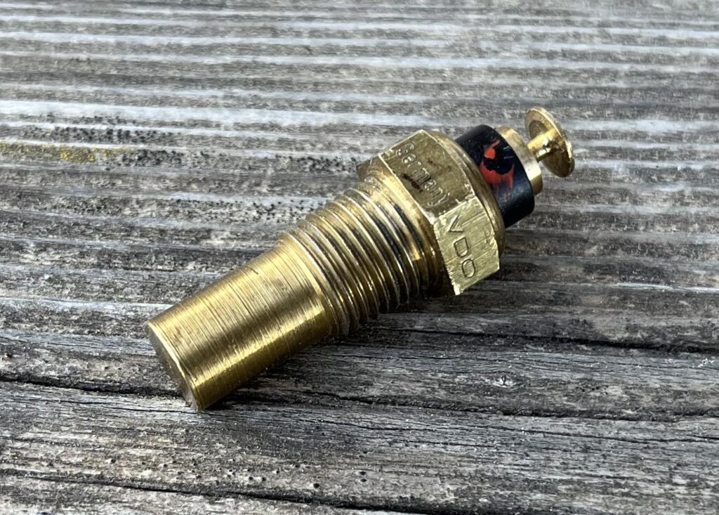
On Rotax engines, VDO brand sensors used for oil temperature, CHT, and waterless coolant temperature (fig. 1) are calibrated for a maximum temperature of 150°C (VDO part #323-057). For conventional coolant (non-waterless) temperature, a VDO sensor calibrated for 120°C (VDO part #323-095) is used.
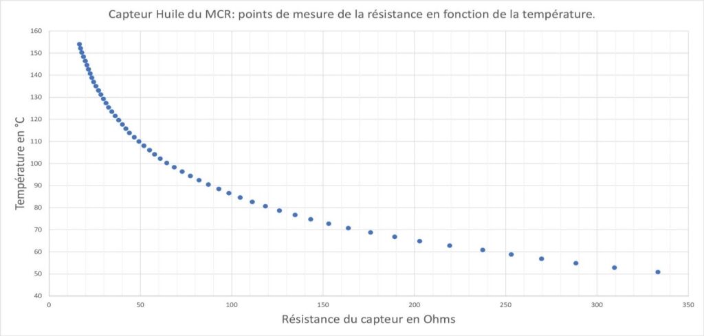
The manufacturer of these sensors does not provide precise information on their characteristics. Therefore, we determined these characteristics by measuring the resistance of these two types of sensors as a function of temperature, from 50°C to 150°C.
Procedure
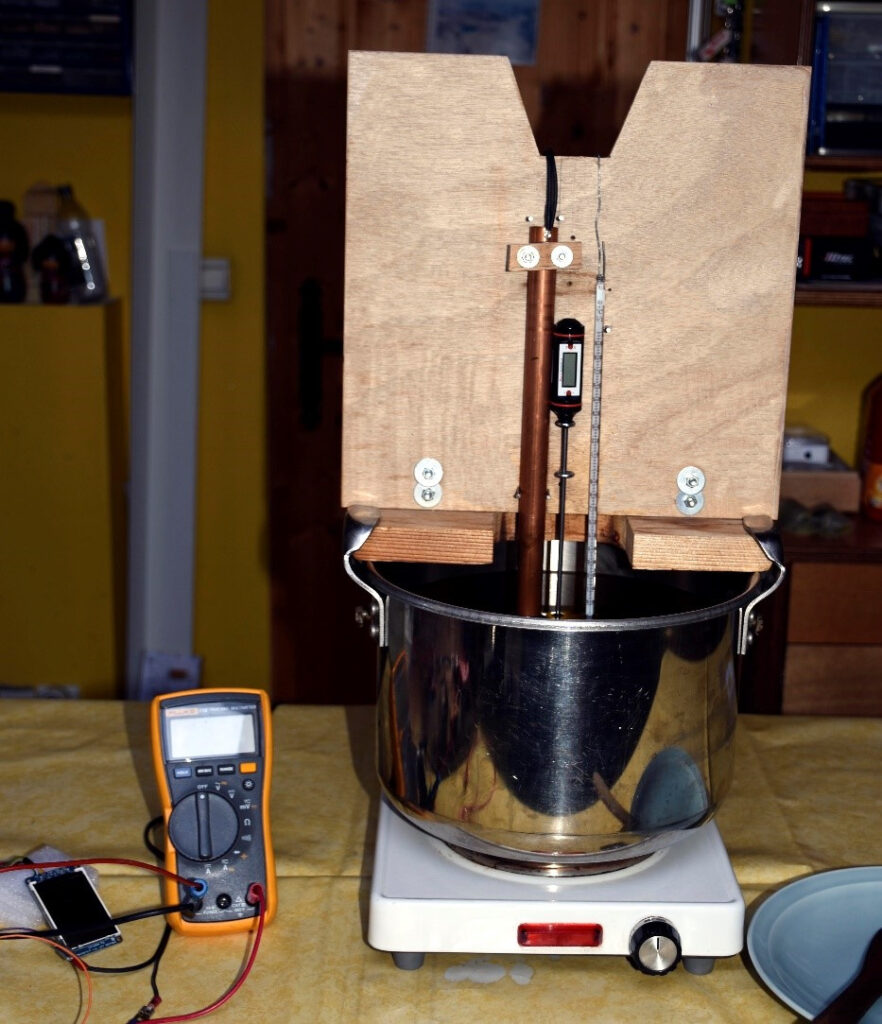
The sensor to be calibrated is immersed in a container filled with oil and heated to 160°C (fig. 2). Then, let cool, constantly stirring to homogenize the temperature. Using an ohmmeter and a digital thermometer previously calibrated against mercury laboratory thermometers, the sensor resistance is noted every 2 degrees, which gives the curve below (fig. 3).
Mathematical modeling
The EMS (Engine Monitoring System) displays the engine parameters, including various temperatures. The EMS must first measure the resistance of the sensors and then calculate the corresponding temperature. Therefore, it is necessary to determine the formula the microcontroller can use to calculate these temperatures.
One could use the above formula of Steinhart-Hart, but determining its coefficients A, B, and C starting from experimental measurements is difficult.
An empirical method can give excellent results using a spreadsheet like Excel. The measurement points are plotted in semi-logarithmic coordinates: natural logarithm of the resistance on the horizontal axis and temperature on the vertical axis(fig 4).
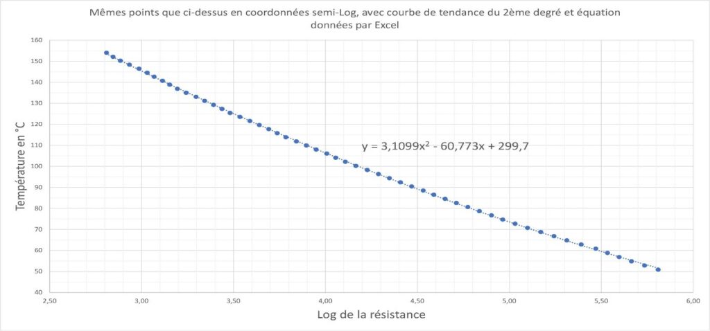
The curve then appears as a conic (polynomial of degree 2). Excel calculates the trendline and its equation shown on the graph (fig. 4). A replacement of the variables is made to obtain the desired formula:
t = A Log(R)2 + B Log(R) + C
The measurements on the two sensor types (VDO-150 and VDO-120) show that these sensors always have almost identical characteristics. A unique formula can perfectly characterize each of the two types.
By taking the average of several sensors of each type, we obtain the following curves and coefficients (fig. 5 and table 1):
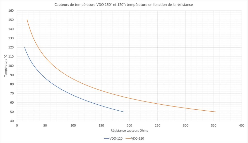
| | A | B | C |
| VDO-150 | 3,193 | -61,72 | 302,2 |
| VDO-120 | -0,796 | -20,39 | 178,8 |
Hi Daniel,
Wishing you a very happy 2026!
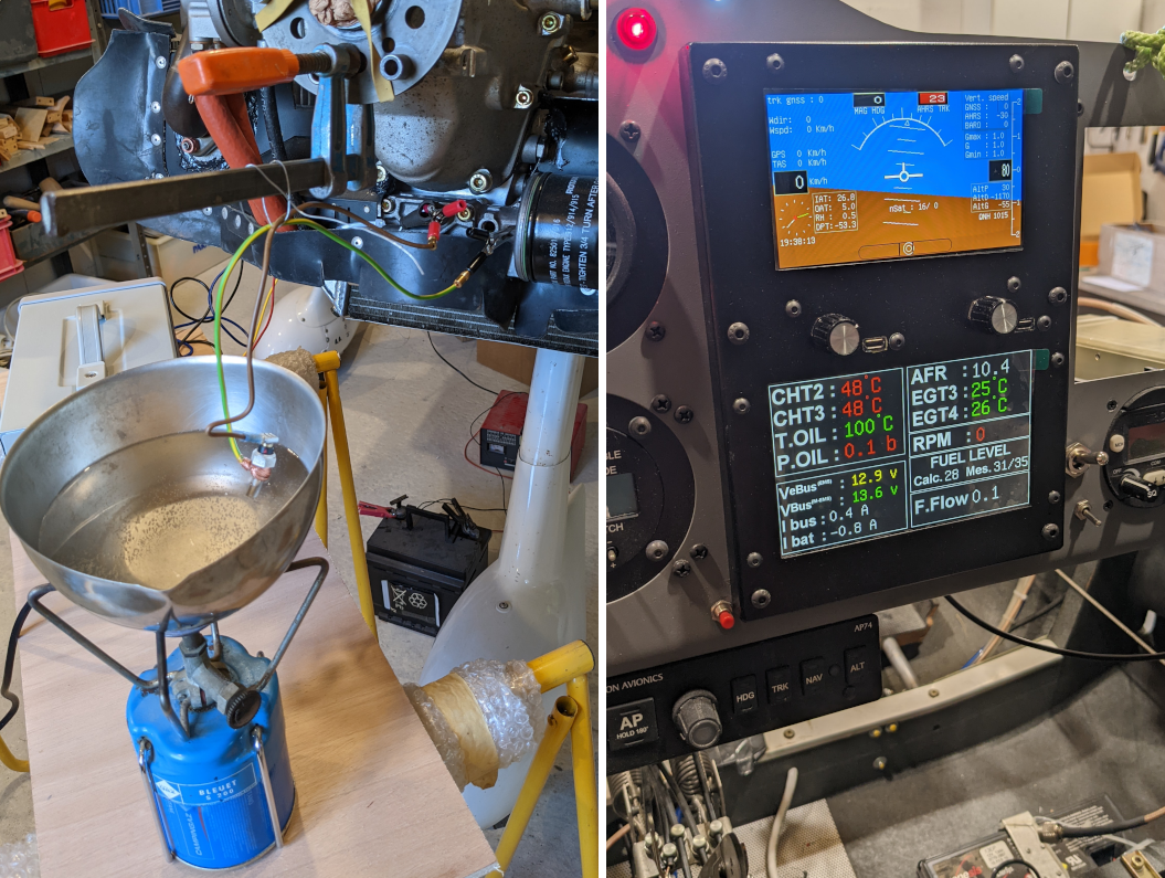
We didn’t consider PT1000 probes for several reasons. We wanted to stick with the standard Rotax configuration. Furthermore, our experiments showed significantly better accuracy than +/-10% with the VDO temperature sensors. In fact, almost as good as +/-1%. The photos below were taken during boiling-water tests (my workroom is 15 ft above sea level, and water boils at exactly 100°C).
These photos show a test with the oil temperature sensor, the EMS on the right indicates an oil temperature of exactly 100 °C. The EGTs, of course, indicate the ambient temperature, while CHT2 and CHT3, although at ambient temperature, indicate 48°C, which is the minimum temperature the electronics can display (a design choice to optimize the measurement range).
In addition, PT1000 probes are generally a bit more expensive and require accounting for the resistance of their connecting wires.
Benjamin
Hi, how are you? For the future EFIS-EMS version, have you considered replacing the Rotax sensors with PT1000 probes? They are available with the same thread and have a margin of error of +1%, while the originals have a margin of error of +/- 10%.
Hi Dermot McD,
Your comment raises various points.
A new cylinder head configuration was introduced on Rotax 912 in 2013 (see service bulletins SB-912-066 / SB-912-066UL).
The temperature probe on the new configuration is no longer in the cylinder head material but in the coolant itself. However, the temperature sensor reference is unchanged: 965531 in the last version (20-12-2024) of the Rotax Illustrated Parts Catalog (IPC) and 965531 in an old IPC version from 2007. The oil temperature sensor shares the same 965531 reference. As far as I know, this Rotax reference corresponds to VDO part #323-057.
A unique sensor reference for CHT (old configuration) and coolant temperature (new configuration) is possible because the measured temperature ranges in both cases are not so different due to liquid cooling of the cylinder heads (the situation is entirely different for an air-cooled engine). So, Rotax has not changed its thinking about temperature sensors, but about their location.
Meters and gauges are indeed another topic. Whether you measure CHT, coolant temperature, or oil temperature, this should be reflected in instrument naming and range limits. These meters must match the sensor’s characteristics. For example, a commercial meter matching VDO sensor #323-057 will display wrong temperatures with VDO #323-095.
Oil pressure sensors have effectively changed, as mentioned on our dedicated page. This page only deals with old sensors because, at the time it was written, we did not have a new Honeywell or Keller sensor at hand.
I do not fully agree with your assertion about the fairly poor accuracy of VDO temperature sensors. Our experimental measurements on several sensors showed, on the contrary, quite satisfactory accuracy and precision. As you pointed out, temperatures below 45-50 °C or above 120-150°C do not concern us, so the input stage of our EMS is optimized for this temperature range. It is very easy to boil water at 1013 HPa atmospheric pressure (100°C) to check the accuracy and precision of the whole sensor-electronic-software system around this critical point. Moreover, our experimental measurements have shown precision and acuracy to the nearest degree for temperatures in the range of 50 to 150°C. Without using the Steinhart-Hart equation, mapping, or any other third-party library. As Gabriel mentioned in the comment just before yours.
Regarding ESP32-based displays, please stay tuned to this website. A new EFIS-EMS using a 7″ ESP32S3 display will soon be published in the “Flight-tested systems” section of the AvionicsDuino website! As a preview, you can see a screenshot in my comment dated March 8, 2025, in the EFIS page comments.
Benjamin
I was looking at this problem recently because the temp sensors in a new 912 Rotax don’t match the old meters where there’sCHT and ammeters on the same meter. I think Rotax have changed their thinking a bit on the sensors too so they are interested in coolant temperature instead of CHT. On new engines the oil pressure sender has changed, perhaps to something more reliable. I think an esp32 based display will do about 10 times as much in the same space… volts, amps, coolant temperature. outside air temperature etc .
I think the VDO sensors are fairly poor in terms of accuracy. The Aviasport oil temperature meter doesn’t read anything below 45ºC. But what do we need to know with any accuracy? It seems to me that we need to know the coolant and oil temperature accurately around boiling point so the water in the oil vaporises but outside this narrow band, it’s not important if the meter reads a few degrees out.
I found a thread about temperature reading and Steinhart-Hart equations where someone mentioned the Multimap library as being a quick and easy way of getting a curve which is accurate where it needs to be. https://github.com/RobTillaart/MultiMap
This should allow me to easily calibrate the sensor and check the accuracy at the important points.
Hi Kirk,
As described in the article about temperature sensors, the method I used is purely experimental and the formula I give results from my trial to best describe the observed variation of resistance versus temperature.
So my formula is completely independent from the Steinhart-Hart Equation which I quoted only for reference. One could derive the Steinhart-Hart Equation coefficients from my exprrimental points, but I did not do that since it would not make the calculation made by the microcontroller easier at all.
And, in addition, my formula happens to give quite accurate results, so I feel it is best to use it as it is.
Unfortunately, I have no experience with Ceres or g2o libraries, so I cannot say wether the problem can be treated with them, but my feeling is that there is no need to look for another method since my curve is accurate enough.
Wishing you a good success in your developments,
Gabriel
Hi Kirk,
I will forward your question to Gabriel, who did the sensor’s experimental measurements, and mathematical modeling, and then wrote this article. His response will be published here soon.
Thanks very much for your interest and careful reading.
Best regards,
Benjamin
Hi Benjamin, the method you proposed for determining sensor model parameters is really impressive. I’m wondering that whether the first formula $/frac{1}{T} = A + BLn(R) + C(Ln(R))^3$ can be or not derived into the second one $t = A Log(R)^2 + B Log(R) + C$ , or is the second one independent from the first?
I once used some C++ libraries named Ceres or g2o to do some calibration of imu and camera or optimization problem, is the above problem worth of being treated similarly?
Best regards,